Gate Execution Quality Metrics#
This tutorial covers benchmarks for measuring quantum gate performance.
from qcmet import CliffordRB, InterleavedRB, OverUnderRotationAngle, CycleBenchmarking
from qcmet.devices import NoisySimulator, IdealSimulator
import matplotlib.pyplot as plt
import numpy as np
The gate execution quality metrics consist of:
Gate set tomography based process fidelity (GST)
Clifford randomised benchmarking (CliffordRB)
Interleaved Clifford randomised benchmarking (InterleavedRB)
Cycle-benchmarking composite process fidelity (CycleBenchmarking)
Over- or under-rotation angle (OverUnderRotationAngle)
Clifford Randomized Benchmarking (RB)#
Clifford Randomized Benchmarking measures the average error rate of a gate set by applying random sequences of Clifford gates.
How Clifford RB Works#
Generate random sequences of Clifford gates of varying lengths
Append an inverse gate to return to |0⟩
Measure success probability
Fit decay curve: P(success) = A × p^m + B
Extract average gate error from decay parameter p
# Create simulator
noisy_device = NoisySimulator()

# Setup CliffordRB benchmark
rb = CliffordRB(
    qubits=2,
    m_list = [25,50,100,150,200,250,300,400,500,650],
    circs_per_m=10
)

# Generate circuits
rb.generate_circuits()
print(rb.config)
print(f"Generated {len(rb.circuits)} circuits")
print(f"Total circuits: {len(rb.config['m_list'])} lengths × {rb.config['circs_per_m']} samples")
{'m_list': [25, 50, 100, 150, 200, 250, 300, 400, 500, 650], 'circs_per_m': 10, 'interleaved_clifford': None}
Generated 100 circuits
Total circuits: 10 lengths × 10 samples
# Look at circuit structure
print("Example RB circuit:")
print(rb.circuits[10])
Example RB circuit:
              ░         ░       ░ ┌────────┐ ░       ░       ░ ┌───┐ ░        »
   q_0: ──────░─────────░───────░─┤0       ├─░───────░───■───░─┤ Z ├─░────────»
        ┌───┐ ░ ┌─────┐ ░ ┌───┐ ░ │  Iswap │ ░ ┌───┐ ░ ┌─┴─┐ ░ └───┘ ░ ┌─────┐»
   q_1: ┤ Z ├─░─┤ Sdg ├─░─┤ Y ├─░─┤1       ├─░─┤ Z ├─░─┤ Y ├─░───────░─┤ Sdg ├»
        └───┘ ░ └─────┘ ░ └───┘ ░ └────────┘ ░ └───┘ ░ └───┘ ░       ░ └─────┘»
meas: 2/══════════════════════════════════════════════════════════════════════»
                                                                              »
«         ░       ░ ┌───┐ ░ ┌───┐ ░       ░     ░ ┌──────┐ ░       ░ ┌───┐ ░ »
«   q_0: ─░───────░─┤ Y ├─░─┤ X ├─░───────░──■──░─┤0     ├─░───────░─┤ X ├─░─»
«         ░ ┌───┐ ░ └─┬─┘ ░ └─┬─┘ ░ ┌───┐ ░  │  ░ │  Ecr │ ░ ┌───┐ ░ └───┘ ░ »
«   q_1: ─░─┤ X ├─░───■───░───■───░─┤ Z ├─░──■──░─┤1     ├─░─┤ Z ├─░───────░─»
«         ░ └───┘ ░       ░       ░ └───┘ ░     ░ └──────┘ ░ └───┘ ░       ░ »
«meas: 2/════════════════════════════════════════════════════════════════════»
«                                                                            »
«              ░       ░ ┌──────┐ ░ ┌───┐ ░       ░ ┌──────┐ ░       ░ ┌───┐ ░ »
«   q_0: ──────░───────░─┤ √Xdg ├─░─┤ X ├─░───────░─┤ √Xdg ├─░───────░─┤ Y ├─░─»
«        ┌───┐ ░ ┌───┐ ░ └──────┘ ░ └───┘ ░ ┌───┐ ░ └──────┘ ░ ┌───┐ ░ └─┬─┘ ░ »
«   q_1: ┤ X ├─░─┤ I ├─░──────────░───────░─┤ I ├─░──────────░─┤ I ├─░───■───░─»
«        └───┘ ░ └───┘ ░          ░       ░ └───┘ ░          ░ └───┘ ░       ░ »
«meas: 2/══════════════════════════════════════════════════════════════════════»
«                                                                              »
«        ┌──────┐ ░       ░       ░ ┌────────┐ ░       ░ ┌───┐ ░       ░      »
«   q_0: ┤1     ├─░───────░───────░─┤0       ├─░───────░─┤ Y ├─░───────░──────»
«        │  Ecr │ ░ ┌───┐ ░ ┌───┐ ░ │  Iswap │ ░ ┌───┐ ░ └─┬─┘ ░ ┌───┐ ░ ┌───┐»
«   q_1: ┤0     ├─░─┤ S ├─░─┤ Z ├─░─┤1       ├─░─┤ I ├─░───■───░─┤ Z ├─░─┤ I ├»
«        └──────┘ ░ └───┘ ░ └───┘ ░ └────────┘ ░ └───┘ ░       ░ └───┘ ░ └───┘»
«meas: 2/═════════════════════════════════════════════════════════════════════»
«                                                                             »
«         ░ ┌──────┐ ░ ┌────┐ ░ ┌───┐ ░ ┌────┐ ░ ┌──────┐ ░       ░     ░ ┌───┐»
«   q_0: ─░─┤0     ├─░─┤ √X ├─░─┤ I ├─░─┤ √X ├─░─┤1     ├─░───────░──■──░─┤ Z ├»
«         ░ │  Ecr │ ░ └────┘ ░ └───┘ ░ └────┘ ░ │  Dcx │ ░ ┌───┐ ░  │  ░ └───┘»
«   q_1: ─░─┤1     ├─░────────░───────░────────░─┤0     ├─░─┤ I ├─░──■──░──────»
«         ░ └──────┘ ░        ░       ░        ░ └──────┘ ░ └───┘ ░     ░      »
«meas: 2/══════════════════════════════════════════════════════════════════════»
«                                                                              »
«         ░ ┌───┐ ░ ┌──────┐ ░ ┌───┐ ░       ░ ┌───┐ ░       ░ ┌────────┐ ░ »
«   q_0: ─░─┤ Y ├─░─┤0     ├─░─┤ Y ├─░───────░─┤ Z ├─░───────░─┤0       ├─░─»
«         ░ └───┘ ░ │  Ecr │ ░ └───┘ ░ ┌───┐ ░ └───┘ ░ ┌───┐ ░ │  Iswap │ ░ »
«   q_1: ─░───────░─┤1     ├─░───────░─┤ Y ├─░───────░─┤ X ├─░─┤1       ├─░─»
«         ░       ░ └──────┘ ░       ░ └───┘ ░       ░ └───┘ ░ └────────┘ ░ »
«meas: 2/═══════════════════════════════════════════════════════════════════»
«                                                                           »
«              ░       ░         ░ ┌──────────┐ ░ ┌─┐
«   q_0: ──■───░───────░─────────░─┤0         ├─░─┤M├───
«        ┌─┴─┐ ░ ┌───┐ ░ ┌─────┐ ░ │  Inverse │ ░ └╥┘┌─┐
«   q_1: ┤ Y ├─░─┤ S ├─░─┤ Sdg ├─░─┤1         ├─░──╫─┤M├
«        └───┘ ░ └───┘ ░ └─────┘ ░ └──────────┘ ░  ║ └╥┘
«meas: 2/══════════════════════════════════════════╩══╩═
«                                                  0  1
# Run benchmark
rb.run(noisy_device, num_shots=1024)

# Analyze
results = rb.analyze()
print("\nRB Results:")
for key, value in results.items():
    print(f"  {key}: {value}")
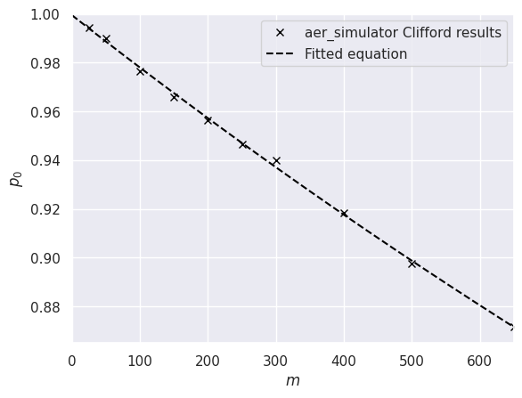
RB Results:
  qubits: 2
  alpha: 0.9996772896169319
  AverageGateError: 0.00024
  fit_result: {'popt': array([0.99967729, 0.67568573, 0.32379839]), 'pcov': array([[ 2.18584749e-08,  4.11562949e-05, -4.12954106e-05],
       [ 4.11562949e-05,  7.75766023e-02, -7.78317533e-02],
       [-4.12954106e-05, -7.78317533e-02,  7.80885979e-02]])}
Visualizing RB Decay#
# Plot
rb.plot()
plt.show()
Comparing Gate Quality#
Let’s compare gate quality between ideal and noisy simulators:
# Run RB on noisy simulator
ideal_device = IdealSimulator()

rb_noiseless = CliffordRB(
    qubits=2,
    m_list = [25,50,100,150,200,250,300,400,500,650],
    circs_per_m=10
)

rb_noiseless.generate_circuits()
rb_noiseless.run(ideal_device, num_shots=1024)

results_ideal = rb_noiseless.analyze()

print("\nComparison:")
print(f"Average gate error ideal: {results_ideal.get('AverageGateError', 'N/A')}")
print(f"Average gate error noisy simulator: {results.get('AverageGateError', 'N/A')}")
Comparison:
Average gate error ideal: -0.00000
Average gate error noisy simulator: 0.00024
What the Numbers Mean#
Average Gate Error: Average gate error of a set of single- and multi-qubit Clifford gates
The lower the Average Gate Error, the better the quality of Clifford operations.
Interleaved Clifford Randomized Benchmarking (RB)#
Interleaved Clifford Randomized Benchmarking measures the average error rate of a target Clifford gate in a gate set. This is done by interleaving a target Clifford gate through random sequences of Clifford gates.
How Interleaved RB Works#
Generate random sequences of Clifford gates of varying lengths
Append an inverse gate to return to |0⟩
Measure success probability
Fit decay curve: P(success) = A × p^m + B
Extract average gate error from decay parameter p
Generate random sequences of Clifford gates of varying lengths interleaved with target Clifford gate
Repeat steps 2-5 to extract the decay parameter p_i for the interleaved circuits.
Calculate interleaved gate error using the decay parameters p and p_i.
from qiskit import QuantumCircuit

# Create simulator
device = NoisySimulator()

# Create circuit with target Clifford gate
circ = QuantumCircuit(1)
circ.x(0)

# Setup interleavedRB benchmark
irb = InterleavedRB(
    qubits=1,
    m_list = [25,50,100,150,200,250,300,400,500,650],
    circs_per_m=10,
    interleaved_clifford=circ
)

# Generate circuits
irb.generate_circuits()
print(irb.config)
print(f"Generated {len(irb.circuits)} circuits")
print(f"Total circuits: {len(irb.config['m_list'])} lengths × {irb.config['circs_per_m']} samples")
{'m_list': [25, 50, 100, 150, 200, 250, 300, 400, 500, 650], 'circs_per_m': 10, 'interleaved_clifford': <qiskit.circuit.quantumcircuit.QuantumCircuit object at 0x7f1403d07380>}
Generated 200 circuits
Total circuits: 10 lengths × 10 samples
# Run benchmark
irb.run(device, num_shots=1024)

# Analyze
results = irb.analyze()
print("\nIRB Results:")
for key, value in results.items():
    print(f"  {key}: {value}")
IRB Results:
  qubits: 1
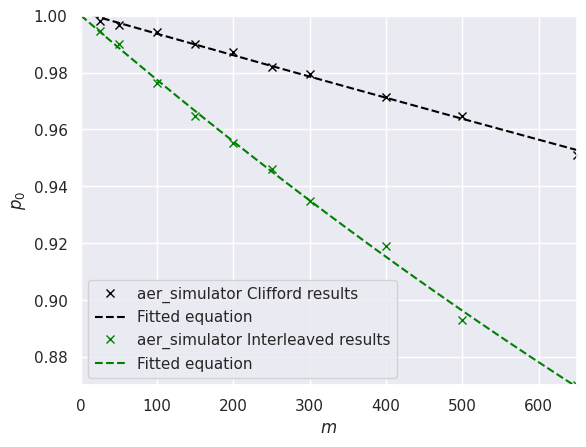
  alpha: 0.9999235760656404
  alpha_g: 0.9995476221471704
  AverageGateError: 0.00004
  InterleavedGateError: 0.00019
  Clifford_fit: {'fit_result': {'popt': array([0.99992358, 1.        , 0.00125025]), 'pcov': array([[ 6.44838319e-08,  8.23109620e-04, -8.23263413e-04],
       [ 8.23109620e-04,  1.05072126e+01, -1.05091647e+01],
       [-8.23263413e-04, -1.05091647e+01,  1.05111175e+01]])}}
  Interleaved_fit: {'fit_result': {'popt': array([0.99954762, 0.51257069, 0.48753614]), 'pcov': array([[ 3.74777624e-08,  3.65497812e-05, -3.67946455e-05],
       [ 3.65497812e-05,  3.57284630e-02, -3.59581700e-02],
       [-3.67946455e-05, -3.59581700e-02,  3.61909435e-02]])}}
Visualizing InterleavedRB Decay#
# Plot
irb.plot()
plt.show()
What the Numbers Mean#
Average Gate Error: Average gate error of a set of single- and multi-qubit Clifford gates
The lower the Average Gate Error, the better the quality of Clifford operations.
Interleaved Gate Error: Average gate error of a target Clifford gate in a gate set
The lower the Interleaved Gate Error, the better the quality of the target Clifford operation.
Over/Under Rotation Angle#
This benchmark detects systematic over-rotation or under-rotation errors in single-qubit gates.
overrotation_amount= np.pi/100
device = NoisySimulator(t1=0, t2=0, overrotation_amount=overrotation_amount)

rotation_exp = OverUnderRotationAngle(
    qubits=1,
    delta_m=5,  # Maximum gate repetitions
)

# Generate and run
rotation_exp.generate_circuits()
print(f"Generated {len(rotation_exp.circuits)} circuits")

rotation_exp.run(device, num_shots=1024)
results_rot = rotation_exp.analyze()

print("\nRotation Analysis Results:")
for key, value in results_rot.items():
    print(f"  {key}: {value}")
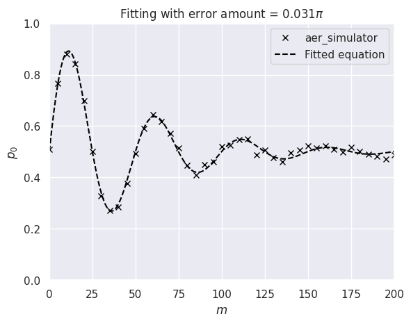
rotation_exp.plot()
Generated 41 circuits

Rotation Analysis Results:
  success: True
  OverUnderRotationAngle: 0.03146251398870455
  fit_result: {'popt': array([ 0.50052081, -0.5020418 ,  0.02107131,  0.12585006,  1.5753996 ]), 'pcov': array([[ 4.51268404e-06,  5.94109362e-06, -2.59998197e-07,
         9.94502958e-08, -2.85527367e-06],
       [ 5.94109362e-06,  1.81765069e-04, -7.86083103e-06,
        -9.72212447e-07,  5.47409729e-05],
       [-2.59998197e-07, -7.86083103e-06,  6.01151691e-07,
         3.84869866e-08, -2.25924771e-06],
       [ 9.94502958e-08, -9.72212447e-07,  3.84869866e-08,
         4.30265278e-07, -8.18183895e-06],
       [-2.85527367e-06,  5.47409729e-05, -2.25924771e-06,
        -8.18183895e-06,  3.98614943e-04]])}
(<Figure size 640x480 with 1 Axes>,
 <Axes: title={'center': 'Fitting with error amount = 0.031$\\pi$'}, xlabel='$m$', ylabel='$p_0$'>)
What the Numbers Mean#
Over/Under Rotation Angle (in radians): The amount of over/under- rotation per gate
A positive value represents an over-rotation by the target gate.
A negative value represents an under-rotation by the target gate.
The larger the magnitude of over/under- rotation, the lower the accuracy of the gate rotation.
Further benchmarks#
Additional gate quality metrics implemented in QCMet are
Gate set tomography based process fidelity (GST)
Cycle-benchmarking composite process fidelity (CycleBenchmarking)
These also follow the standard workflow:
device = NoisySimulator()

# gate layer to benchmark
circ = QuantumCircuit(2)
circ.h(0)
circ.cx(0, 1)
circ.x(1)

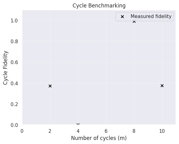
cyclebm = CycleBenchmarking(circ, [2, 4, 8, 10])

cyclebm(device)
{'composite_process_fidelity': {'m=2_to_m=4': 4.03307128518151,
  'm=2_to_m=8': 1.1263552467649778,
  'm=2_to_m=10': 0.5437854647893269,
  'm=4_to_m=8': 0.49965640854839666,
  'm=4_to_m=10': 0.5190481243612284,
  'm=8_to_m=10': 0.40691147471081385},
 'method': 'ratio',
 'success': True,
 'ptm_elements': {2: {'XX': 0.99765625,
   'XY': 0.0185546875,
   'XZ': 0.00625,
   'XI': 0.015234375,
   'YX': 0.998046875,
   'YY': 0.0009765625,
   'YZ': -0.016015625,
   'YI': 0.99921875,
   'ZX': 0.9974609375,
   'ZY': -0.019140625,
   'ZZ': -0.0017578125,
   'ZI': -0.0140625,
   'IX': 0.998828125,
   'IY': 0.0033203125,
   'IZ': -0.007421875},
  4: {'XX': 0.9947265625,
   'XY': -0.9947265625,
   'XZ': -0.9947265625,
   'XI': 0.994921875,
   'YX': 0.996875,
   'YY': -0.9943359375,
   'YZ': -0.9951171875,
   'YI': 0.9962890625,
   'ZX': 0.9958984375,
   'ZY': -0.9955078125,
   'ZZ': -0.994140625,
   'ZI': 0.99375,
   'IX': 0.99765625,
   'IY': -0.994921875,
   'IZ': -0.9947265625},
  8: {'XX': 0.9927734375,
   'XY': 0.9880859375,
   'XZ': 0.989453125,
   'XI': 0.99296875,
   'YX': 0.9931640625,
   'YY': 0.9923828125,
   'YZ': 0.9880859375,
   'YI': 0.99140625,
   'ZX': 0.992578125,
   'ZY': 0.987109375,
   'ZZ': 0.990234375,
   'ZI': 0.991796875,
   'IX': 0.9935546875,
   'IY': 0.98828125,
   'IZ': 0.9890625},
  10: {'XX': 0.9896484375,
   'XY': -0.003515625,
   'XZ': 0.0013671875,
   'XI': 0.01484375,
   'YX': 0.9890625,
   'YY': -0.001171875,
   'YZ': -0.005859375,
   'YI': 0.9908203125,
   'ZX': 0.9904296875,
   'ZY': 0.0138671875,
   'ZZ': 0.0025390625,
   'ZI': 0.0025390625,
   'IX': 0.991015625,
   'IY': -0.00078125,
   'IZ': 0.01875}},
 'cycle_fidelities': [0.37357177734375,
  0.0007446289062499958,
  0.99130859375,
  0.37459716796875]}