Quickstart Guide

This tutorial provides a quick introduction to using QCMet for quantum computing benchmarks.

Running a T1 Measurement

To run a benchmark in QCMet, two main things are required:

1. A benchmark, defining a specific set of circuits to be run on a device together with the analysis instructions

2. An interface to a device which is benchmarked.

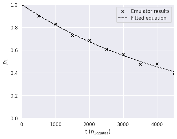
Here we consider a simple T1 measurement. T1 is the relaxation time of a qubit - the time it takes for an excited state to decay to the ground state.

The easiest way to run the T1 benchmark on a device (here an emulator with noise) is as follows:

from qcmet import T1
from qcmet.devices import NoisySimulator
device = NoisySimulator()
t1_benchmark = T1()
result = t1_benchmark(device=device, num_shots=1000, max_circs_per_job=None)
print(result)

{'success': True, 'T1 (t/t_[1q_gate])': np.float64(5041.365580956495), 'fit': {'popt': array([1.00130568e+00, 5.04136558e+03]), 'pcov': array([[ 1.28255647e-04, -1.23537721e+00],
       [-1.23537721e+00,  2.11534629e+04]])}}

Workflow Summary

Under the hood, benchmarking in QCMet follows the same pattern:

1. Create a device (simulator or real hardware)

2. Initialize the benchmark with parameters

3. Generate circuits using generate_circuits()

4. Run on device using run(device, num_shots, max_circs_per_job)

5. Analyze results using analyze() and plot()

This consistent interface makes it easy to swap between different benchmarks and devices.

Steps 3., 4., and 5. are bundled together via the call function of the benchmark, allowing the above workflow.

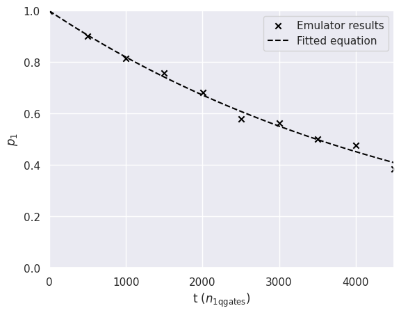
The extended version of the above looks as follows (giving more fine-grained control over the workflow):

device = NoisySimulator()
t1_benchmark = T1()
t1_benchmark.generate_circuits()
t1_benchmark.run(device, num_shots=1000, max_circs_per_job=None)
t1_benchmark.analyze()

print(t1_benchmark.result)

# Optional plotting
t1_benchmark.plot();

{'success': True, 'T1 (t/t_[1q_gate])': np.float64(5037.61158501775), 'fit': {'popt': array([9.99471683e-01, 5.03761159e+03]), 'pcov': array([[ 1.47857787e-04, -1.42490332e+00],
       [-1.42490332e+00,  2.44154351e+04]])}}

Running a Collection of (Different) Benchmarks

Using BenchmarkCollection, (different) benchmarks can be conveniently collected together and run in one go. The workflow for BenchmarkCollection is the same.

from qcmet import BenchmarkCollection, T2, CliffordRB

t1_benchmark_1 = T1(qubit_index=0)
t1_benchmark_2 = T1(qubit_index=1)
t2_benchmark_1 = T2(qubit_index=0)
t2_benchmark_2 = T2(qubit_index=1)
rb_benchmark_1 = CliffordRB([2 ** n for n in range(1, 11)], qubits=[0, 1])
rb_benchmark_2 = CliffordRB([2 ** n for n in range(1, 11)], qubits=[2, 3])

collection = BenchmarkCollection({"T1_qubit0": t1_benchmark_1, "T1_qubit1": t1_benchmark_2,
                                  "T2_qubit0": t2_benchmark_1, "T2_qubit1": t2_benchmark_2,
                                  "RB_qubit01": rb_benchmark_1, "RB_qubit23": rb_benchmark_2})

# Using the same workflow
collection.generate_circuits()

"""
Now there are two different ways to run the circuits

When passing in a list of shot number for num_shots, all the circuits are submitted
to the device one after the other and each benchmark is run separately with the
corresponding number of shots:
"""
# collection.run(device, num_shots=[1000 for _ in range(6)])

"""
When passing in a single number for num_shots, all circuits are merged and submitted
as one batch
"""
collection.run(device, num_shots=1000)

collection.analyze()
collection.plot()

# Or directly use the call function
# collection(device, num_shots=1000)

print(collection.result)

{'T1_qubit0': {'success': True, 'T1 (t/t_[1q_gate])': np.float64(5135.319546014731), 'fit': {'popt': array([1.00406397e+00, 5.13531955e+03]), 'pcov': array([[ 4.63538808e-05, -4.60218624e-01],
       [-4.60218624e-01,  8.08647860e+03]])}}, 'T1_qubit1': {'success': True, 'T1 (t/t_[1q_gate])': np.float64(4929.84554576347), 'fit': {'popt': array([1.00404889e+00, 4.92984555e+03]), 'pcov': array([[ 9.65397941e-05, -8.91066505e-01],
       [-8.91066505e-01,  1.47018583e+04]])}}, 'T2_qubit0': {'success': True, 'T2 (t/t_[1q_gate])': np.float64(3006.4763888036273), 'method': 'hahn', 'fit': {'popt': array([2.45147572e-01, 3.00647639e+03, 7.56375161e-01]), 'pcov': array([[ 6.76609479e-03,  1.14795553e+02, -6.96666209e-03],
       [ 1.14795553e+02,  1.97505744e+06, -1.18662514e+02],
       [-6.96666209e-03, -1.18662514e+02,  7.18292297e-03]])}}, 'T2_qubit1': {'success': True, 'T2 (t/t_[1q_gate])': np.float64(1781145.3340818333), 'method': 'hahn', 'fit': {'popt': array([ 1.14228013e+02,  1.78114533e+06, -1.13228696e+02]), 'pcov': array([[ 2.20654162e+09,  3.44247690e+13, -2.20654182e+09],
       [ 3.44247690e+13,  5.37068837e+17, -3.44247721e+13],
       [-2.20654182e+09, -3.44247721e+13,  2.20654202e+09]])}}, 'RB_qubit01': {'qubits': 2, 'alpha': 0.9997803691805811, 'AverageGateError': '0.00016', 'fit_result': {'popt': array([9.99780369e-01, 1.00000000e+00, 2.34461082e-04]), 'pcov': array([[ 1.36693837e-08,  5.59801336e-05, -5.60568878e-05],
       [ 5.59801336e-05,  2.29509200e-01, -2.29812914e-01],
       [-5.60568878e-05, -2.29812914e-01,  2.30118480e-01]])}}, 'RB_qubit23': {'qubits': 2, 'alpha': 0.999659271964362, 'AverageGateError': '0.00026', 'fit_result': {'popt': array([0.99965927, 0.6618    , 0.33802598]), 'pcov': array([[ 9.40928673e-09,  1.54997037e-05, -1.55508867e-05],
       [ 1.54997037e-05,  2.56083545e-02, -2.56879253e-02],
       [-1.55508867e-05, -2.56879253e-02,  2.57687010e-02]])}}}

Implemented benchmarks

QCMet ships various benchmarking protocols for (digital) quantum computers:

Qubit Quality Metrics

• T1: Relaxation time (energy decay)

• T2: Relaxation time (dephasing)

• Idle Qubit Oscillation Frequency: Non-Markovian noise induced coherence revivals

Gate Execution Quality Metrics

• Clifford RB: Average gate error rate

• Interleaved RB: Specific gate error rate

• Over/Under Rotation: Systematic rotation errors

• Cycle Benchmarking: Average fidelity of a repeated layer

• Gate Set Tomography: Full characterization of process fidelity

Circuit Execution Quality Metrics

• Quantum Volume: Holistic circuit complexity measure

• Mirrored Circuits: Target circuit performance benchmark

• Upper Bound on Variation Distance: Quantum accreditation protocol

Well-studied Task Execution Quality Metrics

• QFT: Quantum Fourier Transform fidelity

• VQE: Energy expectation value reproducibility

• QScore: Metric based on using QAOA for a MaxCut problem

• Hamiltonian Simulation: Ability to perform Hamiltonian dynamics